This Appendix provides background to enable users of the standard (building owners, lenders, insurance brokers, etc.) and service providers (engineers and risk consultants) to make effective use of the standard.
A1. Event Sets
A2. Building Damage Models
A3. Value Estimation
A4. Other Risks
A5. Risk Aggregation Methods
A6. Stakeholder Allocation Models
A7. Limitations to the State of the Art
A1. Event Sets
The objective of portfolio seismic risk assessment is to find the losses to a geographically distributed group of real estate properties in future earthquakes. Some researchers have attempted to develop ways to combine the risks from geographically separated sites based on correlation of risks found using single-site methods, e.g., [Wesson et al., 2009]. Such methods can provide estimates for the “ground-up” losses for a portfolio in a particular region, but they have greater difficulty addressing losses to stakeholders such as insurers, where insurance deductibles apply event-by-event. They also typically do not address the effects of spatial correlation of ground shaking and loss in large-to-great earthquakes, where the source fault rupture may be tens to hundreds of kilometers long. A more common approach is to simulate individual potential earthquakes one at a time, each one with its spatial distribution of ground shaking and other hazards. In the past, some real estate lenders tracked portfolio-wide losses for a few selected maximal scenarios, such as magnitude 8 events on the San Andreas in northern or southern California, but focusing on any individual scenario may lead to poor decisions on particular properties, and will not provide adequate guidance on earthquake insurance needs. Over the past several decades, as led by insurance catastrophe modelers, losses are now evaluated for comprehensive sets of earthquake simulations in a balanced, probabilistic approach.
In the most common probabilistic approach to multi-site seismic risk assessment, portfolio losses are computed for a comprehensive set of earthquake simulations (or scenarios), sometimes referred to as an ‘event set.’ Each event or earthquake simulation attempts to accurately reproduce the geographic distribution of ground shaking and other hazards from a possible future earthquake. The ground motion simulations estimate ground motion intensity parameters (i.e., peak ground acceleration, or spectral acceleration) at each property site in the portfolio for each potential future earthquake with the associated event probabilities or annual frequency.
Since geographic correlation of damage is of primary concern in the seismic risk assessment of a geographically distributed system, the physical size of the source rupture must be properly modeled. The affected area is modeled with an appropriate ground motion attenuation relationships. Each event is associated with an annual frequency of occurrence (a number of events per year, typically << 1), where the annual frequencies are derived from fault activity, magnitude and fault rupture location “sampling.” The ‘event set’ systematically exercises the full range of earthquake magnitudes and rupture locations for each seismic sources, including known faults and background seismicity. The set of scenarios is carefully constructed so that the ensemble accurately reproduces the severity and frequency of earthquake hazards for the region of interest. These simulations usually involve thousands or even millions of scenarios in each complex tectonic region, such as southern California, where numerous known and unknown faults exist and produce frequent earthquakes.
Ground motion models for portfolio risk assessment are typically derived from, and attempt to conform to, the National Seismic Hazard Mapping Project by the United States Geological Survey [e.g., Frankel et al, 1996, 2002; or Peterson et al., 2008, 2014]. The National Seismic Hazard Mapping Project is an ongoing national program that utilizes the seismologists, geotechnical engineers and other experts of the USGS as well regional experts to assess earthquake hazards based upon the best available science. This sustained scientific effort (1996, 2002, 2008, 2014…) has produced substantial improvements in the knowledge of and prediction of earthquake activities and ground shaking hazards in the U.S., and is widely emulated around the world. As the National Seismic Hazard Mapping Project is the source for the maps used in all design codes for new buildings to resist seismic loads, as well as for the standards (e.g., ASCE 41) used in the evaluation of existing buildings, the USGS seismic hazard model represents the de facto national standard.
In selecting and appropriate catastrophe model for use in portfolio analysis, the Service Provider may wish to request documentation that compares or demonstrates the conformance of ground shaking hazards produced by the ensemble of simulations in the event set to the current USGS National Seismic Hazard Mapping Project model. See Section 2.3. The comparison should address the Intensity Measures (IMs) used by the damage models to be used (i.e., spectral acceleration, or Sa), spanning the range of structural periods of interest (0s to 5s or more) and the return periods of interest (e.g., 100 years to 1,000 years).
Ground motion models such as the NGA West 2 models [PEER, 2013] segregate the aleatory uncertainty in ground shaking estimates into inter-event and intra-event terms. Inter-event (or “between event”) uncertainty in ground shaking manifests in systematically higher or lower ground shaking throughout the affected area that occurs from earthquake to earthquake, whereas intra-event (or “within event”) variability in ground shaking that occurs from site-to-site within the same earthquake. The inter-event uncertainty of ground shaking causes correlated changes in ground shaking and hence loss throughout the portfolio, producing significant changes in aggregate loss, whereas intra-event uncertainty of ground shaking causes locally correlated changes in ground shaking [Baker and Jayaram; Goda & Hong], with more limited impacts on portfolio-wide loss. Such distinctions are not relevant in single-site seismic risk assessments, but are important in portfolio analysis. The hazard model “event set” and the component vulnerability models for buildings and contents must carefully manage the uncertainties, capture their effects but avoid double-counting.
A1.1 Uncertainties in Ground Motions and Relevance to Portfolio Risk
A1.1.1 Types of Uncertainty
One common way to classify uncertainty in mathematical models of physical process is to distinguish between aleatory and epistemic uncertainties. Aleatory uncertainties are associated with the inherent randomness of a physical process, and this randomness is often quantified by a statistical distribution. For example, the uncertainty in ground motion models (attenuation relationships) are assumed to have a lognormal distribution. In contrast, epistemic uncertainty – also called scientific uncertainty – is more concerned with the adequacy of our understanding of the physics underlying the process and the adequacy of existing models of the process.
A1.1.2 Aleatory Uncertainty
Re-write to address uncertainty in each major part: exposure ($$, time, people), hazards, vulnerability and repair cost (adjustment or construction).
In estimating the statistical distribution of financial losses from each ground motion simulation, all of the uncertainties must be carefully tracked and accounted for. Some earthquake damage models (e.g., HAZUS) may include consideration of ground motion uncertainties in computing damage state probabilities or repair costs. Catastrophe modelers must be careful not to neglect, nor to double-count the uncertainties.
A1.1.3 Epistemic Uncertainty
The development of an earthquake risk catastrophe model requires selection from among multiple admissible component models – for asset valuation, for ground shaking and other hazards, for damageability, and for the aggregation and allocation of losses or other consequences. No component model is perfect, and comprehensive approaches may incorporate logic trees or other methods to manage the uncertainty arising from the use of multiple component models. Differences arising from multiple admissible scientific models is referred to as epistemic uncertainty.
Methods such as Robust Simulation [Taylor, C.E., 2015] preserve and present this epistemic uncertainty, which can be substantial. This is important to recognize, so that results from such complex models are not viewed as precise. Furthermore, it is clear that as new findings emerge, new models will be formulated, so any current model must be regarded as incomplete.
A2. Building Damage Models
Given any ground shaking simulation for the portfolio, the hazards at each of the individual sites are estimated, and vulnerability or fragility models are then used to estimate the damage and other consequences to the individual properties at those sites. Portfolio-wide risks may then be found, using aggregation techniques that consider the uncertainties in the building-by-building and site-by-site losses.
A2.1 Damage Inception and Damage Saturation
It is important to note that, unlike seismic risk assessment for individual buildings where risks are reported for a defined scenario such as the 475-year probabilistic ground shaking, damage relationships used for portfolio seismic risk assessment must accurately predict damage for the the full range of hazard levels. During the evaluation of losses for a comprehensive set of earthquake simulations (the “event set”), the damage relationship will be interrogated at all hazard levels, and aggregations of loss may include many locations with low levels of damage, some with moderate or high levels of damage, and (typically) a few locations with complete or near-complete loss. Hence the damage relationships used for portfolio seismic risk assessment should have appropriate behavior throughout the range of damage, from damage inception to saturation.
A2.2 Overview of Building Damage Models
Depending on the damage model to be used, different data must be collected for portfolio seismic risk studies.
Available models may be classified as expert-based, statistical, empirical, or engineering-based (either lumped-parameter or explicit).
An example of a published statistical model is [Wesson, 2004]. ATC-13 [Applied Technology Council, 1985] is drawn from expert opinion sampled at Modified Mercalli Intensities, using defined Facility Classes. The Code-Oriented Damage Assessment model (or CODA) [Graf & Lee, 2009] is an example of empirical damage model, but where damage is a function of a demand-to-capacity ratio in terms of engineering parameters. HAZUS [Kircher, 1997] is another example of an engineering-based model, although model parameters are often expert-based.
Commercial catastrophe modelers have developed their own proprietary damage models. Some are based upon building usage (termed ‘occupancy’) for use when structural characteristics are not known. Other damage models are based upon the structural systems and materials used. These structurally-based models can be made more building specific using attributes often referred to as secondary modifiers, such as soft-story or torsional irregularity.
A2.3 Insurance Taxonomies
Taxonomies in insurance earthquake damage models generally rely on attributes and externally observable features (age, height, occupancy), that are readily available or may be determined without the involvement of engineers, with the result that they do not achieve maximum correlation with damage, nor minimize the prediction variance. An example of earthquake insurance inventory reporting categories is the system published by the Insurance Services Office (ISO), and still used by the California Department of Insurance (CDI).
A2.4 Structural Building Classification Systems (Structural Taxonomies)
Structural building classification systems or structural taxonomies are used to group buildings with similar earthquake damage characteristics, for the purpose of loss estimation. Such groupings are needed when examining loss experience data, and should be based on relevant observable or readily-determined building characteristics. Because they consider the building systems designed to resist earthquake loading, structural taxonomies are assumed to achieve higher correlation with damage, and to minimize the prediction variance, compared to taxonomies that are not based on the lateral force-resisting system.
Location and age may be used to determine the code under which a building was designed and constructed, and can be used to account for local design and construction, inspection and enforcement practice. Other relevant and effective information includes height or height class, materials of construction of floors and roof (wood, steel, concrete), and earthquake resisting system (braced frame, moment frame, shear wall) and materials of construction (wood, steel, concrete, masonry).
A3. Value Estimation
Building replacement values, contents values and costs per unit time resulting from functional interruption are generally supplied by the property owner or broker. Damage models for individual buildings usually predict damage or loss as a fraction of replacement value. To obtain dollars losses, the loss rates are multiplied by replacement values, so any errors in value translate directly to errors in risk results. Care must be exercised in estimating the values, to be consistent with stakeholder position. For instance, a commercial building owner may own only the building shell and may not own or be responsible for damage to tenant contents or tenant improvements. Therefore the building and other values used for estimating losses must focus on the exposure of the particular stakeholders whose risks are to be examined.
Commercial systems may be used for value estimation. Valuation consultants may also be useful. Costs for business interruption may be estimated by individual business units for the enterprise in question. Insurance brokers may also be able to offer guidance.
A4. Other Risks
Additional loss or damage may occur due to the temporary increase in repair costs that occurs following large regional earthquakes (“demand surge” or “loss amplification”), damage to contents and architectural building elements caused by earthquake-induced leakage of fire sprinkler piping (or “EQSL” for earthquake sprinkler leakage), or earthquake-initiated fires (“fire-following” damage). Each catastrophe model offers a different approach to modeling these additional loss or damage elements.
A5. Risk Aggregation Methods
Models that assume that aggregate losses conform to a particular statistical distribution (e.g., a normal, lognormal, or Pareto distribution) may be subject to significant errors where insurance deductibles and limits (or other risk “buffers” related to stakeholder position) affect the shape of losses for individual properties, and these errors may compound for higher stakeholder positions (as encountered in reinsurance). Aggregation methods based on statistical sampling strategies, similar to Monte Carlo methods, when properly applied, produce more reliable estimates of aggregate loss distributions.
A6. Stakeholder Allocation Models
For each earthquake simulation in an “event set”, a hazard model predicts the ground shaking intensity (i.e., PGA, spectral acceleration) at each site, and damage models then estimate the damage level for each building, given the earthquake hazard intensity predicted. There is significant uncertainty in the prediction of the ground-shaking intensity. Ground motion uncertainties may be modeled using a lognormal distribution as published for attenuation relationships (e.g., NGA West2, [PEER]), for instance by binning the intensity into a large number of hazard states, each with a specified probability. Furthermore, for each hazard state, the actual loss for any type of building may vary from a predicted mean loss. Building damage models generally predict repair cost as a fraction of the building replacement value, so the uncertainty in the repair cost, in dollars, is a function of the uncertainty in the damage model and (as appropriate) the uncertainty in estimated replacement values.
Given these uncertainties, for any earthquake “event,” the loss for any property can be represented using statistical distributions. The cost to repair a building may vary from zero to a repair cost equal to the full replacement value of the building. The statistical distribution of the loss can be subdivided into bins, and the loss in each bin allocated to the stakeholders according to stakeholder logic as described below.
A6.1 Insurance Loss Model
Insurance may cover costs to repair buildings, costs to replace damaged contents, costs related to downtime or business interruption, or costs related to temporary relocation while repairs are effected. For insured properties, losses are allocated between the insured party (typically the owner) and the insurer. The insurer may in turn cede a portion of their risks to one or more reinsurers.
A typical insurance policy uses stated deductibles and limits to determine the portion of the loss retained by the insured and the portion paid by the insurer. A minimum deductible may be specified, as well as a per unit deductible, usually stated as a percentage of the property replacement value. For costs related to business interruption, the deductible may be specified as a period of time. Limits of coverage are generally specified for portfolio-wide losses to buildings, to contents and/or time-element (downtime) losses.
Insurance loss allocation models operate on the statistical loss distributions for building damage, for contents damage and for losses from downtime or business interruption to allocate the losses between the insured party and the insurer. Deductibles and limits apply typically per event (that is, per earthquake) with the “event” defined by a period of time. If an aftershock occurs after the main shock and outside the time window used to define the event, an addition deductible would apply.
A6.2 Lender Loss Model
The lender for a property will not be affected by earthquake losses unless the borrower (owner) defaults on the mortgage. The lender is protected by the owner’s equity (and any owner-retained earthquake insurance).
A stakeholder loss allocation diagram for the lender loss depicted in the figure below. The vertical axis (in dollars) denotes building value at the left and a statistical distribution of loss at the right. The market value of the property is composed of the replacement value building(s) and the value of the land.
The figure illustrates the normal mortgage case, with positive equity (i.e., market value exceeds mortgage balance). That is, the loan-to-value ratio (LTV) is less than one. For low levels of loss (just above the zero dollars axis), repair costs are below owner equity. For such losses, the owner may repair the damage, and continue to make mortgage payments. Alternatively, the owner may sell the property, pay off the mortgage and recoup the equity remaining after the cost of repairs. When losses exceed owner equity, the owner may choose to default on the mortgage. In this case, the lender may repair the structure and sell the property at market value, with a loss equal to:
Lender Loss = Mortgage Balance + Earthquake Repair Cost – Market Value (Salvage)
Note that when market value falls below the mortgage balance, the owner has no equity. In lender terms, the loan-to-value ratio exceeds 100%, and (presumably) default becomes much more likely.
The lender model accounts for the variability of the damage prediction using statistical distributions and easily accommodates declines in the real estate market. The model can be run at full current market value and at any specified fraction of the market value (representing an assumed level of market value decline).
If the owner has earthquake insurance, the earthquake insurance coverage amount acts like additional owner equity. The earthquake insurance payments offset repair costs, with any earthquake deductible coming out of the owner’s equity.
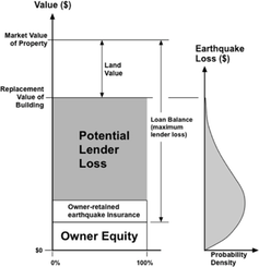
Lender Loss Model
A7. Limitations to the State of the Art
Conventional risk models may not adequately consider cumulative earthquake effects on urban regions, for instance due to impacts from lifeline disruption, and due to collateral impact from the collapses of tall buildings in urban areas.
References for the Technical Appendix
ATC 13. Earthquake Damage Evaluation Data for California, ATC-13, Applied Technology Council, Redwood City, California, 1985.
Baker, J.W. and Jayaram, N., Correlation of Spectral Acceleration Values from NGA Ground Motion Models. Earthquake Spectra: Vol. 24, No. 1, February 2008.
Goda, K. and Hong, H. P., Spatial Correlation of Peak Ground Motions and Response Spectra, Bulletin of the Seismological Society of America, Vol. 98, No. 1, pp. 354–365, February 2008.
Graf, W.P., and Y. Lee, “Code-Oriented Damage Assessment for Buildings,” EERI Spectra Journal, Vol. 25, No. 1, February, 2009.
Kircher, C.A., Nassar, A.A., Kustu, O. and Holmes, W.T., “Development of Building Damage Functions for Earthquake Loss Estimation,” Earthquake Spectra, Vol. 13, No. 4, November 1997.
PEER 2013/04, 05, 06, 07, 08, Pacific Earthquake Engineering Research Center, available at: https://peer.berkeley.edu/peer-reports
Taylor C.E, “Robust Simulation For Mega-Risks - The Path from Single Solutions to Competitive, Multi-Solution Methods for Mega-Risk Management,” Springer International Publishing, ISBN 978-3-319-19413-4, October, 2015.
Wesson, R.L., Perkins, D.M., Leyendecker, E.V., Roth, Jr., R.R., and Petersen, M.D., “Losses to Single-Family Housing from Ground Motions in the 1994 Northridge, California, Earthquake” Spectra, August, 2004.
Wesson, R.L., Perkins, D.M., Luco, N. and Karaca, E., Direct Calculation of the Probability Distribution for Earthquake Losses to a Portfolio, Earthquake Spectra, Earthquake Engineering Research Institute, 2009.